More examples
Motorcyle data
This is a classic dataset featuring unknown heteroscedastic noise.

Motorcycle dataset.
The noise increases near 10 and 30. We model it with our TGP.
"""
Classic motorcycle data example
===============================
"""

import numpy as np
import matplotlib.pyplot as plt

import kingpin as kp


# Data and points for prediction

x, y = np.loadtxt("motorcycle.txt", unpack=True)
p = np.linspace(x.min(), x.max(), 301)

# Bespoke choices

model = kp.Celerite2(x, y, x_predict=p)

# Priors and proposals for mean, sigma, length and nugget

mean = kp.Uniform(-200., 150.)
sigma = kp.Uniform(0., 500.)
length = kp.Uniform(0., 50.)
nugget = kp.Uniform(0., 300.)
params = kp.Independent(mean, sigma, length, nugget)

# Run RJ-MCMC

rj = kp.TGP(model, params)
rj.walk(thin=10, n_threads=4, n_iter=20000, n_burn=2000, n_iter_params=1, screen=False)

# Examine results

print(rj.acceptance)
print(rj.arviz_summary())

plt.scatter(x, y)
plt.xlabel('Time (ms)')
plt.ylabel('Acceleration ($g$)')
plt.savefig("motorcycle_data.png")

rj.plot()
plt.savefig("motorcycle_tgp.png")
The result correctly models the heteroscedastic noise in the distinct regions.
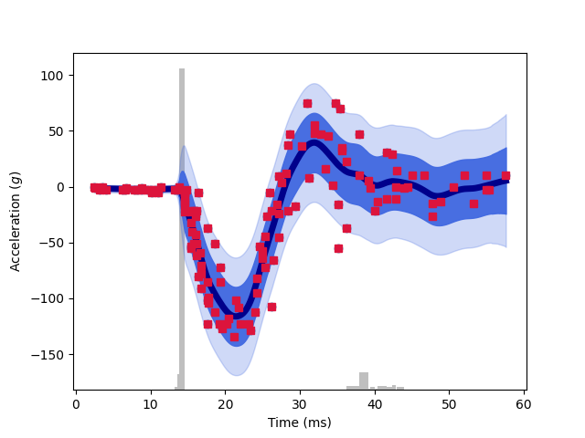
TGP model of motorcyle dataset. The grey bars show the locations of partitions.
Step-functions
The data contains step-functions, which ordinary GPs struggle with.
"""
Example with step-functions
===========================
"""

import numpy as np
import matplotlib.pyplot as plt

import kingpin as kp


# Data and points for prediction

x = np.linspace(0, 10, 51)
truth = 100. * np.ones_like(x)
truth[x > 5.05] = 500.
truth[x > 7.55] = 100.
noise = 10 * np.ones_like(x)
y = truth + np.random.randn(*x.shape) * noise
p = np.linspace(x.min(), x.max(), 201)

# Bespoke choices

model = kp.Celerite2(x, y, noise, p)

# Priors and proposals for mean, sigma and length

mean = kp.Uniform(0., 750.)
sigma = kp.Uniform(0., 750.)
length = kp.Uniform(0., 10.)
params = kp.Independent(mean, sigma, length)

# Run RJ-MCMC

rj = kp.TGP(model, params)
rj.walk(n_threads=None, n_iter=1000, n_burn=500)

# Examine results

print(rj.acceptance)
print(rj.arviz_summary())

plt.xlabel('$x$')
plt.ylabel('$y$')
rj.savefig("step_functions_tgp.png")
The step is modeled appropriately by the TGP:
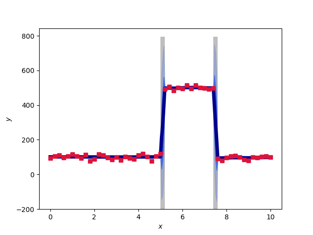
TGP model of step functions. The grey bars show the locations of partitions.